Physics Overview

The present code implements a Four-Dimensional T′ Expansion Scheme (4D-TExS) to construct a QCD equation of state (EoS) that depends on temperature \(T\) and three independent chemical potentials: baryon \(\mu_B\), electric charge \(\mu_Q\), and strangeness \(\mu_S\). This code was written following the method described in Ref. [1].

Compared to traditional Taylor expansion methods (limited to \(\mu/T \lesssim 2.5–3\)), the 4D-TExS allows for extrapolation up to \(\mu/T \sim 3.5\) in the direction of the baryon chemical potential, extending the usable region of the QCD phase diagram significantly. This method relies on a change of coordinates and a local rescaling of temperature using generalized susceptibilities computed from continuum-estimated lattice data and HRG results.

The T′-expansion scheme is based on the observation that the dependence of certain fluctuation observables on baryon chemical potential \(\mu_B\) can be effectively captured by a chemical-potential-dependent shift in temperature.

In the 2D case (involving only \(T\) and \(\mu_B\)), presented in [2], the expansion is defined through:

\[\frac{n_B(T,\hat{\mu}_B)}{\hat{\mu}_B} = \chi_2^B(T') \, ,\]

where \(\hat{\mu}_B = \mu_B/T\) and the redefined effective temperature \(T'\) absorbs the \(\mu_B\) dependence:

\[T'(T,\hat{\mu}_B) = T \left(1 + \kappa_2^B(T) \hat{\mu}_B^2 + \ldots \right)\]

The coefficient \(\kappa_2^B(T)\) is related to standard Taylor coefficients by:

\[\kappa_2^B(T) = \frac{1}{6 T \, \partial_T \chi_2^B(T)} \chi_4^B(T)\]

An improved version of the scheme considers normalization by the infinite-temperature (Stefan–Boltzmann) limits to encode correct high-temperature behavior [3]:

\[\frac{F(T,\hat{\mu}_B)}{\overline{F}(\hat{\mu}_B)} = \frac{F(T_F',0)}{\overline{F}(0)} \quad , \quad T_F' = T \left(1 + \lambda_{2,F}(T) \hat{\mu}_B^2 + \ldots \right)\]

with:

\[\lambda_{2,F}(T) = \frac{1}{6 T \, \partial_T \chi_2^B(T)} \left( \chi_4^B(T) - \frac{\overline{\chi_4^B}}{\overline{\chi_2^B}} \chi_2^B(T) \right)\]

This approach motivates the generalization to three chemical potentials by treating the expansion as a local coordinate transformation. In 4D-TExS, the effective temperature becomes direction-dependent in \((\mu_B, \mu_Q, \mu_S)\) space, and the expansion remains valid as long as the redefined temperature remains a monotonic function of \(T\).

Change of Coordinates

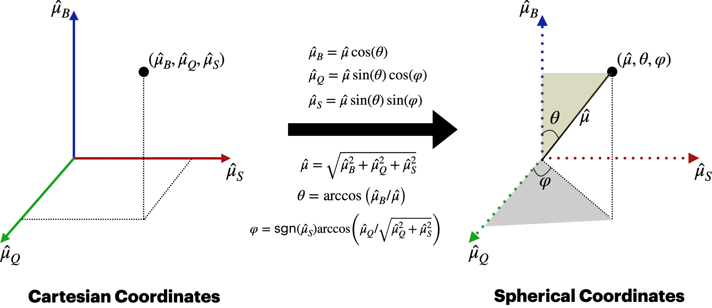
To generalize the T′-expansion to three chemical potentials, we transform the cartesian space of chemical potentials:

\[\left( \hat{\mu}_B, \hat{\mu}_Q, \hat{\mu}_S \right) = \left( \frac{\mu_B}{T}, \frac{\mu_Q}{T}, \frac{\mu_S}{T} \right)\]

into spherical coordinates:

\[\hat{\mu}_B = \hat{\mu} \cos\theta,\quad \hat{\mu}_Q = \hat{\mu} \sin\theta \cos\phi,\quad \hat{\mu}_S = \hat{\mu} \sin\theta \sin\phi\]

This allows one to perform a 1D extrapolation in the radial direction \(\hat{\mu}\), keeping the direction (θ, φ) fixed.

T′ Expansion Scheme

For each chosen direction (θ, φ), we define an effective temperature \(T'\) as a function of \(T\) and \(\hat{\mu}\):

\[T'_{\theta,\phi}(T, \hat{\mu}) = T \left(1 + \lambda_{(2)}^{\theta,\phi}(T) \hat{\mu}^2 \right)\]

The coefficient \(\lambda_{(2)}^{\theta,\phi}(T)\) is determined using susceptibilities:

\[\lambda_{(2)}^{\theta,\phi}(T) = \frac{1}{6T} \left( \frac{d X_2^{\theta,\phi}(T)}{dT} \right) \left( \frac{X_4^{\theta,\phi}(T) - X_4^{\theta,\phi}(0)}{X_2^{\theta,\phi}(0) \, X_2^{\theta,\phi}(T)} \right)\]

The second- and fourth-order susceptibilities along a direction (θ, φ) are:

\[\begin{split}X_2^{\theta,\phi}(T) = \chi_2^B \cos^2\theta + \chi_2^Q \sin^2\theta \cos^2\phi + \chi_2^S \sin^2\theta \sin^2\phi \\ + 2 \cos\theta \sin\theta \cos\phi \, \chi_{11}^{BQ} + 2 \cos\theta \sin\theta \sin\phi \, \chi_{11}^{BS} + 2 \sin^2\theta \cos\phi \sin\phi \, \chi_{11}^{QS}\end{split}\]

A similar expression applies for \(X_4^{\theta,\phi}\) using fourth-order susceptibilities.

The generalized density in the direction (θ, φ) is then written as:

\[X_1^{\theta,\phi}(T, \hat{\mu}) = \frac{X_1^{\theta,\phi}(\hat{\mu})}{X_2^{\theta,\phi}(0)} \cdot X_2^{\theta,\phi}(T'_{\theta,\phi}, 0)\]

This allows the extraction of thermodynamic observables along each direction from purely \(\mu=0\) data.

Susceptibilities

Second- and fourth-order susceptibilities \(\chi_{ijk}^{BQS}(T)\) at zero chemical potential, which are the base ingredients of this expansion, are constructed using a smooth combination of HRG model results (for \(T < 135\) MeV) and continuum-estimated lattice QCD data using 4stout action [1]. These are available up to \(T = 800\) MeV, and are smoothly interpolated across the whole temperature range [4].

All susceptibilities are directionally combined into generalized forms \(X_2^{\theta,\phi}\) and \(X_4^{\theta,\phi}\) as above.

Limits of Applicability

This method is valid as long as the mapping \(T \to T'_{\theta,\phi}\) remains monotonic. When the slope \(dT'/dT\) becomes negative, the expansion breaks down. The maximal range of \(\hat{\mu}\) is direction-dependent but generally reaches up to \(\hat{\mu} \sim 3.5\). Detailed explanations on the applicability of the expansion and its thermodynamics stability is provided in the section on Limits of applicability.

In any direction of the four-dimensional phase diagram, the code will print a warning if the extrapolation is attempted beyond the limit of applicability, and will skip the calculation for that point.

Thermodynamics at Finite Chemical Potential

Using the above procedure, thermodynamic quantities such as pressure, entropy density, energy density, and conserved charge densities can be computed analytically at finite \((\mu_B, \mu_Q, \mu_S)\) by selecting a direction and applying the T′ expansion scheme.

Plots of these quantities versus \(T\) for fixed values of \(\hat{\mu}\) show consistency with HRG at low temperatures and smooth extrapolation to the lattice regime.

References

[1] (1,2)

1. Abuali et al., preprint https://arxiv.org/abs/2504.01881 (2025)

[3]

19. Borsanyi et al., Phys.Rev.Lett. 126, 232001 (2021), https://arxiv.org/abs/2102.06660

[2]

19. Borsanyi et al., Phys.Rev.D 105, 114504 (2022), https://arxiv.org/abs/2202.05574

[4]

Continuum-estimated susceptibilities from lattice QCD, https://doi.org/10.5281/zenodo.15123622